Bulk RNA-seq (9): Gene Ontology Analysis of Differential Expression
Note
Next, we will perform Gene Ontology (GO) to unearth the biological processes, cellular components, and molecular functions our significant genes are involved in. Here’s how we perform a GO analysis on our list of significant genes identified from the DESeq2 analysis.
Reading and Preparing the Data:
# Load the significant gene results, which are in ENSEMBL ID format
degs1 <- read.csv("sig_res.csv", row.names = 1)
head(degs1)  # Display the first few lines to verify the content
In this code, we’re loading the sig_res.csv file which contains the significant genes listed by their ENSEMBL IDs.
Gene Ontology Analysis with clusterProfiler:
# Loading the necessary packages for GO analysis
library(org.Hs.eg.db)
library(clusterProfiler)
library(ggplot2)
library(org.Mm.eg.db)

# Performing the enrichment analysis
ego <- enrichGO(
  gene = degs1$X,
  OrgDb = org.Mm.eg.db,          # Specifying the organism database for mouse
  ont = "ALL",                   # Analyzing all three ontology categories (BP, CC, MF)
  pAdjustMethod = "BH",          # Adjusting p-values using the Benjamini-Hochberg method
  minGSSize = 10,                # The minimum size of genes for a GO term to be considered
  pvalueCutoff = 0.01,           # The threshold for p-value significance
  qvalueCutoff = 0.01,           # The threshold for q-value significance
  keyType = 'ENSEMBL',           # The type of gene ID provided, here ENSEMBL
  readable = TRUE                # Convert the ENSEMBL IDs to readable gene names
)

# Save the enriched GO results to a CSV file
write.csv(as.data.frame(ego), "GO_all_enrich.csv", row.names = FALSE)
We utilize the clusterProfiler package, a powerhouse in bioinformatics, to conduct GO enrichment analysis on our set of differentially expressed genes. The org.Mm.eg.db package is chosen as it contains the necessary annotations for mouse genes. The parameters are fine-tuned to ensure we capture the most relevant GO terms associated with our dataset.
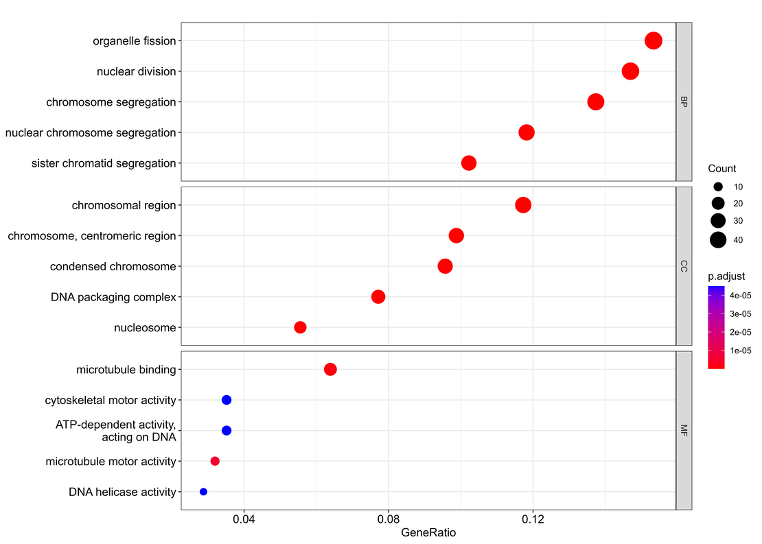
Visualizing the Results with a Dotplot:
# Creating a dotplot to visualize the enriched GO terms
a <- dotplot(ego, split = "ONTOLOGY", showCategory = 10) + facet_grid(ONTOLOGY ~ ., scale = "free")
a  # Print the plot to the R plotting window

# Saving the GO dotplot as a high-resolution image
ggsave("gof.png", a, units = "cm", width = 30, height = 30, dpi = 1200)
The dotplot function from clusterProfiler is adept at showcasing the most significant GO terms, elegantly partitioned by ontology categories, and providing a scalable view across BP (Biological Process), CC (Cellular Component), and MF (Molecular Function). The result is a visually informative plot, ready to guide us through the functional significance of our gene list.