Bulk RNA-seq (6): Normalization and PCA Visualization in RNA-seq Data Analysis with DESeq2
Note
In this blog post, we’ll dive into a practical guide on using DESeq2 for differential expression analysis in RNA-seq data. DESeq2 is a powerful R package designed for analyzing count-based NGS data like RNA-seq and ChIP-seq. Let’s break down the steps and code snippets used in this analysis:
How DESeq2 Calculates DEGs
DESeq2, published in 2014 and cited over 30,000 times, is a method for differential analysis of count data. It utilizes shrinkage estimation for dispersions and fold changes, enhancing the stability and interpretability of estimates. (Reference )
Library Normalization in DESeq2 (Median of Ratios Method)
Unlike RPKM, FPKM, TPM, and other methods that adjust for differences in overall read counts among libraries, DESeq2 employs a unique approach. It addresses:
- Differences in library sizes
- Differences in library composition (e.g., liver vs. spleen)
DESeq2’s median of ratios method normalizes for sequencing depth and RNA composition with a straightforward user experience but involves multiple backend steps:
Step 1: Creating a Pseudo-Reference Sample (Row-wise Geometric Mean)
For each gene, a pseudo-reference sample is calculated as the geometric mean across all samples.
| Gene ID | Sample1 | Sample2 | pseudo-reference |
|---|---|---|---|
| 1 | 1489 | 906 | sqrt(1489 * 906) = 1161.5 |
| 2 | 22 | 13 | sqrt(22 * 13) = 17.7 |
| … | … | … | … |
For instance, the pseudo-reference for Gene 1 is calculated as: $$ \sqrt{1489*906} $$ Notice: If any count data equals 0, the pseudo-reference becomes 0, regardless of other counts.
Step 2: Calculating Ratios to the Reference
For each gene, the ratio of each sample’s count to the pseudo-reference count is calculated.
| Gene ID | Sample1 | Sample2 | pseudo-reference | ratio of sample1/ref | ratio of sample2/ref |
|---|---|---|---|---|---|
| Gene 1 | 1489 | 906 | 1161.5 | 1489/1161.5 = 1.28 | 906/1161.5 = 0.78 |
| Gene 2 | 22 | 13 | 16.9 | 22/16.9 = 1.30 | 13/16.9 = 0.77 |
| … | … | … | … |
Step 3: Determining the Normalization Factor (Size Factor) for Each Sample
The median of all ratios for each sample is determined and used as the normalization factor for that sample. This method assumes that not all genes are differentially expressed, making it robust to imbalances in gene regulation and large numbers of DEGs.
normalization_factor_sample1 <- median(c(1.28, 1.3, ...))
normalization_factor_sample2 <- median(c(0.78, 0.77, ...))
Notice: Size factors are typically around 1.
Step 4: Calculating Normalized Count Values
| Gene ID | Sample1 | Sample2 |
|---|---|---|
| Gene 1 | 1489 / 1.3 = 1145.39 | 906 / 0.77 = 1176.62 |
| Gene 2 | 22 / 1.3 = 16.92 | 13 / 0.77 = 16.88 |
| … | … | … |
Normalized counts are calculated by dividing the original counts by the sample’s normalization factor. This process emphasizes moderately expressed genes over genes that consume a large proportion of reads.
Therefore, additional normalization before using DESeq2 is not necessary as DESeq2’s method effectively accounts for key variables affecting RNA-seq data.
Using DESeq2 for normalization
Preprocessing: Cleaning Up the Data
Before diving into differential expression analysis, it’s crucial to clean up your data. This includes removing genes with zero reads across all samples, as they won’t contribute to the analysis.
# Delete genes whose reads are all 0
mycounts1 <- mycounts[rowSums(mycounts) != 0,]
By doing this, we ensure that the dataset only contains genes that have been expressed in at least one sample.
Setting Up the Experiment Metadata
Metadata contains information about your samples, such as conditions, treatments, or any relevant experimental groups. Correctly inputting this information is vital for the analysis.
# Input metadata
mymeta <- read.table("metadata.txt", stringsAsFactors = TRUE, header = TRUE)
Ensure that the sample names in your metadata match the column names of your count data:
# Check whether sample names match
colnames(mycounts1) == mymeta$Sample
Installing and Loading DESeq2
DESeq2 is available through Bioconductor, and here’s how you can install and load it:
# Installation of DESeq2 package
install.packages("BiocManager")
BiocManager::install("DESeq2")

# Load DESeq2
library(DESeq2)
Preparing the DESeq2 Dataset
Creating a DESeq dataset object (dds) is the first step in your differential expression analysis, linking your count data with the experimental metadata.
dds <- DESeqDataSetFromMatrix(countData = mycounts1,
                              colData = mymeta,
                              design = ~Group)
If you’re interested in comparing a specific group against a reference, you can set your reference group like this:
# Setting the reference level for comparisons
dds$Group <- relevel(dds$Group, ref="WT")
Normalizing the Data
Normalization is key to making fair comparisons between samples. DESeq2 does this using size factors:
dds <- estimateSizeFactors(dds)
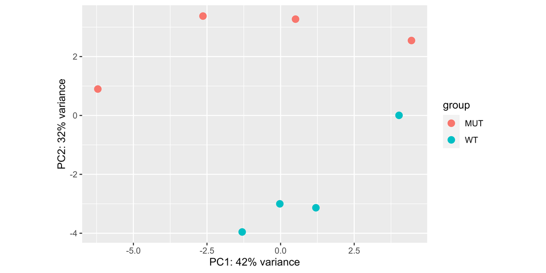
Visualizing Data with PCA
Principal Component Analysis (PCA) is a useful tool for visualizing the overall effect of treatments or conditions on your samples.
library(ggplot2)
rld <- rlog(dds, blind = TRUE)

pca <- DESeq2::plotPCA(rld, intgroup = "Group")
pca

ggsave("PCA.png", units = "cm", width = 20, height = 10, dpi = 1200)